Page 201 - GuideFWA

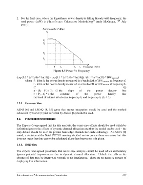
2. For the final case, where the logarithmic power density is falling linearly with frequency, the
total power (mW) is (“Interference Calculation Methodology” Andy McGregor, 7th July
1997):

Power density (P dBm)

P1
P3

P4
P2

f1 f3 f4 f2 Frequency (MHz)

Figure 1.5 Power Vs Frequency

(exp[0.1 * (a*f4+b) * ln(10)] – exp[0.1 * (a*f3+b) * ln(10)]) / (0.1 * a * ln(10) * BWmeasure)
where P1 dBm is the power density measured in a bandwidth of BWmeasure at frequency f1
P2 dBm is the power density measured in a bandwidth of BWmeasure at frequency f2
(f1 < f2)
a = (P2 – P1) / (f2 – f1) the slope of the power density line
b = P1 – f1 * a the constant of the power density line
the band of interest is between frequency f3 and frequency f4 (f3 < f4)

1.3.1. Consensus View

AENS [6] and LMNQ [4, 15] agree that proper integration should be used and the method
advocated by Nortel [4] and corrected by Alcatel [6] should be used.

1.4. PHS TO DECT INTERFERENCE

The Experts Group agreed that for this analysis, the worst-case effects should be used which by
definition ignores the effects of dynamic channel allocation and thus the model can be used – the
only debate should be over the precise band edge channels for each technology. As AENS [6]
noted, a decision at the Natal PCC.III meeting decided not to pursue these scenarios, but this
does not mean that they cannot be calculated given that the process is in place.

1.4.1. LMNQ View

The experts had agreed previously that worst case analysis should be used which deliberately
ignores potential improvements due to dynamic channel allocation. Unlock the cells as the
absence of data may be interpreted wrongly as no interference. There are no negative aspects of
displaying this information.

Inter-American Telecommunication Commission 187